Tests for the Regression Line
- Is there a correlation?
| H0 | r=0 | b=0 |
|---|---|---|
| H1 | r≠0 | b≠0 |
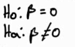
Is the y intercept = 0
H0: a = 0
H1: a ≠ 0
Conditions for Hypothesis Testing
Linearity
- Linear relationship between x and y
Constant Variability (homoscedasticity)
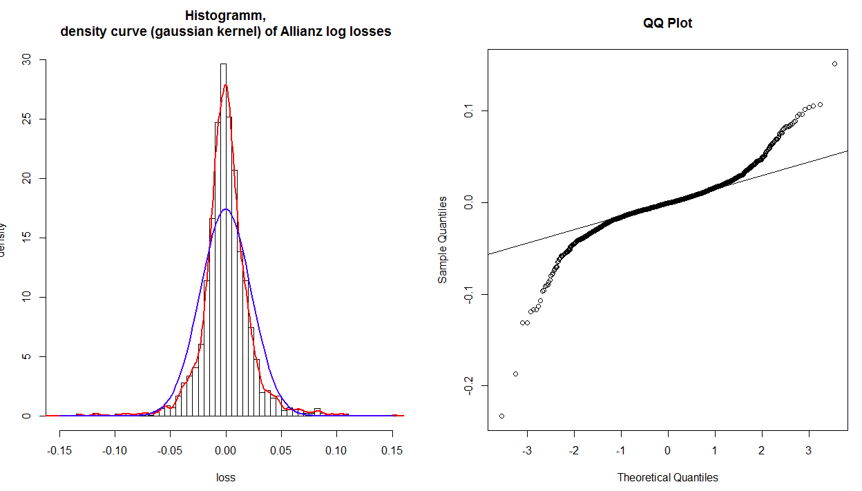
Normality
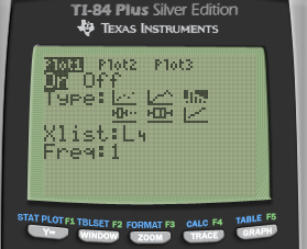
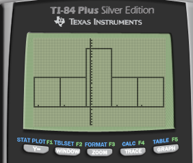
- The residuals should be normally distributed (from Histogram and QQ plot)
Independence
- All the Y are independent
Hypothesis Testing
Practice Question 1
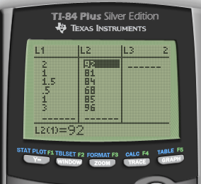
A teacher asked her students to record the total amount Of time they spent studying for a particular test.
The amounts of study time x (in hours) and the resulting test grades y are given below
| x | 2 | 1 | 1.5 | 0.5 | 1 | 3 |
|---|---|---|---|---|---|---|
| y | 92 | 81 | 84 | 68 | 85 | 96 |
Obtain the equation of the least-squares regression line and the correlation.
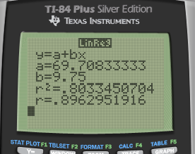
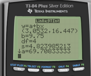
y = 69.7 + 9.75x
r = 0.896 (strong correlation)
r2 = 0.803 (80.3% of the change in grade can be explained by the study time)
Explain in words what the slope b of the least-squares line says about hours studied a nd grade awarded.
- For every 1 hour increase in study time, the grade is expected to go up by 9.75 points
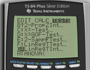
Test the hypothesis that the amount of study time is correlated to the test grade
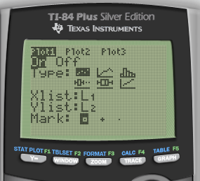
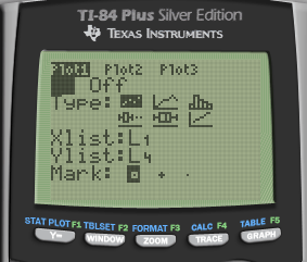
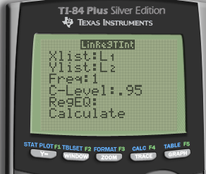
- Data
| L1 | L2 | L3 | L4 |
|---|---|---|---|
| x | y | y hat | Residual |
Hypothesis
Conditions
- Linearity

Constant Variance

Normal Residuals
Independence: each observation is independent
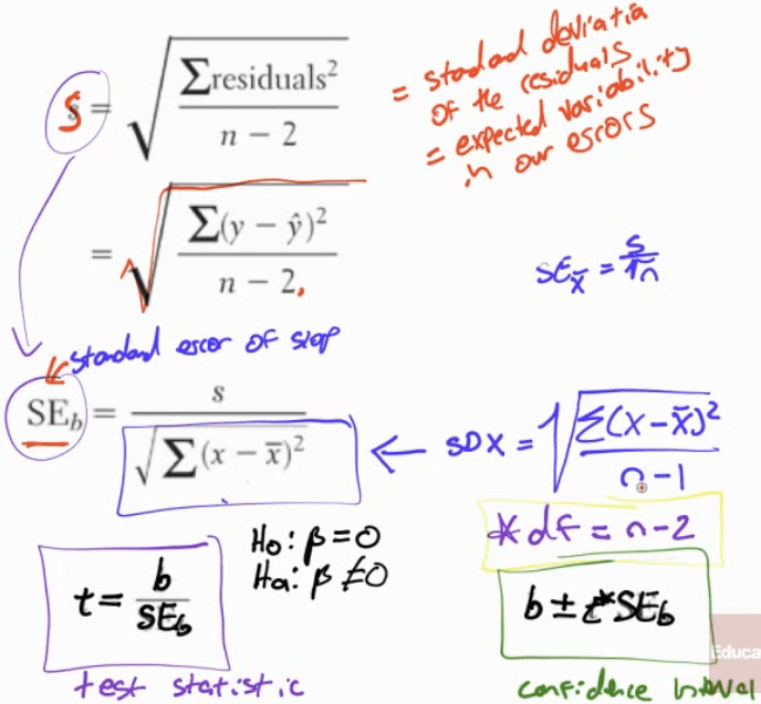
Calculate
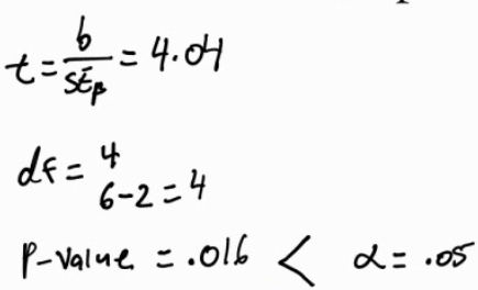
Interpret
- So we reject the null hypothesis and have evidence to support the claim that the slope is not equal to zero. There is a correlation between study time and test grades
What is the 95% confidence interval of the slope?
- Equation
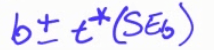
- Calculate
Interpret
- We are 95% confident that on average, for every 1 hour increase in study time, the final grade will go up between 3.05 and 16.45 points
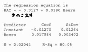
Interpreting Computer Output
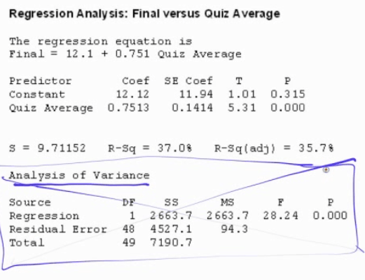
Practice Question 2
An economics professor wishes to analyze whether a person's income can predict the cost of their car
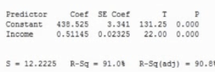
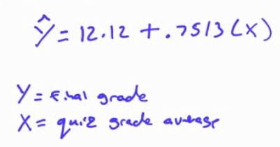
What's the least-squares regression equation
y hat = 438.535 + 0.511 * x
y = cost of car
x = income
What is the standard error about the line (aka the standard deviation of the regression model)? Interpret this value in context
- On average, we expect our prediction of cost is off by 12.22.
Interpret the slope of the least-squares regression line in the context of this problem
- For every $1 increase in income, car cost increases, on average, $0.51
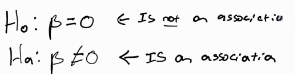
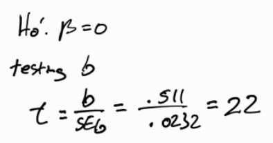
What are the null and alternative hypotheses to test if there is an association between income and car cost?
What is the value of the test statistic for testing the hypotheses
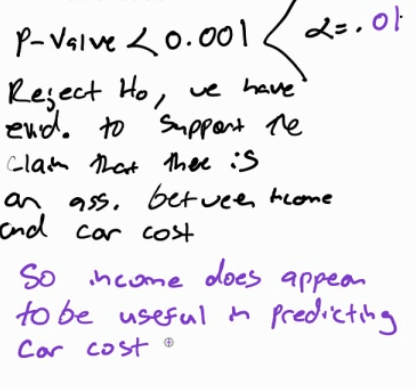
What is the P-value for the test
- P < 0.001
Is income useful for predicting the cost of a person's car? Use a significance level of 0.01. Explain briefly
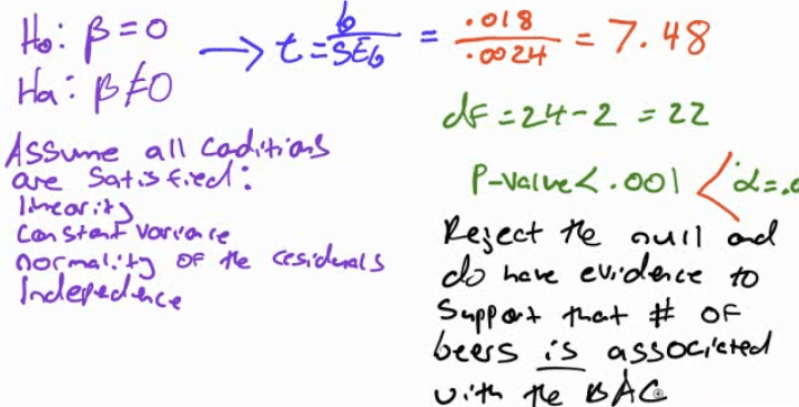
Practice Question 3
Test if the number of beers is associated with the BAC