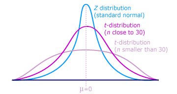
T Distribution
When do we use the T distribution
Know the mean
Do not know the population SD
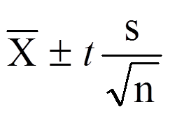
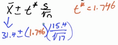
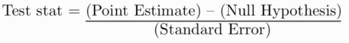
Formula
Degrees of freedom (df)
- df = n-1
Confidence Interval Example
The super Corporation manufactures a device they claim "may increase gas mileage by 23%"
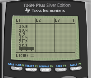
Here are the percent changes in gas mileage for 17 identical vehicles, as presented in one of the company's advertisements
| 48.3 | 46.9 | 46.8 | 44.6 | 40.2 | 38.5 |
|---|---|---|---|---|---|
| 34.6 | 33.7 | 28.7 | 28.7 | 24.8 | 10.8 |
| 6.9 | 12.4 | 21.2 | 25.2 |
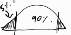
Construct and interpret a 90% confidence interval to estimate the mean fuel savings in the population of all such vehicles.
Type in the data
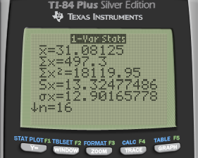
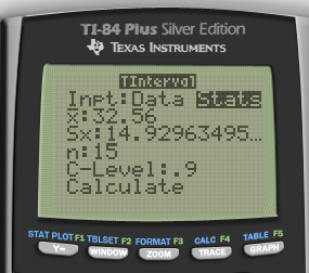
1-Var Stats for the sample
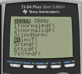
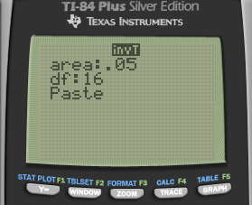
Looking for t
Calculate
Calculate by calculator
Interpret
We are 90% confident that the mean percent change in gas mileage is between 24.68% and 38.16%
Since 23% is in the interval, it appears that the machine does even better than 23% savings
Hypothesis Test Example
When the manufacturing process is working properly, the batteries have lifetimes that follow a right-skewed distribution with µ = 10 hours. A quality control statistician selects a simple random sample of n = 20 batteries every hour and measures the lifetime of each.
If she is convinced that the mean lifetime of all batteries produced that hour is less than 10 hours at the 5% significance level, then all those batteries are discarded.
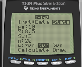
The current sample of 20 has a mean of 8.5 and a SD of 3, should this batch be discarded?
Hypothesis
H0: µ = 10
H1: µ < 10
Conditions
Random: given
Independent: N > 10n = 200
Normal: not larger than 30, but still ok since we are using a T distribution
Calculate
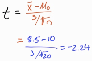
Calculate by calculator

P-value
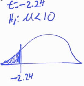
df = n - 1 = 19
Interpret
- Because p < α, we reject the null hypothesis. Thus, we do have evidence to support the claim that the mean battery life in this whole batch is less than 10 hours and so should be discarded
Matched Pairs T-Test
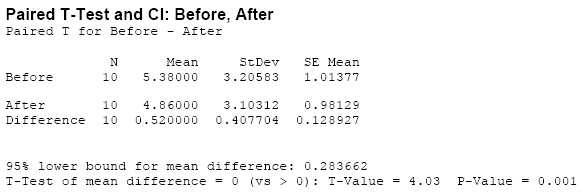
The average weekly loss of study hours due to consuming too much alcohol on the weekend is studied on 10 students before and after a certain alcohol aware ness program is put into operation. Do the data provide evidence that the program was effective?
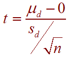
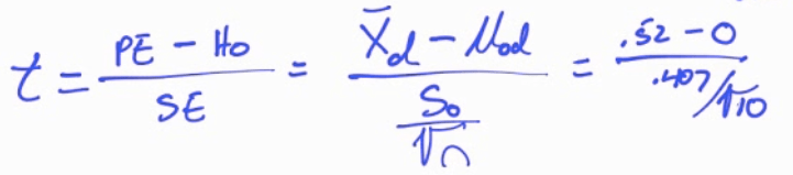
Formula
Data
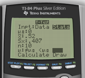
N=10
Difference of mean = 0.52
Difference of SD = 0.407
Hypothesis (d = before - after)
H0: µd = 0
H1: µd > 0
Conditions
Random: assume random selection
Independence: N > 10n = 100
Normal: t-distribution
Calculate
Calculate by calculator

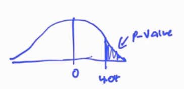
P-value
- df = 10-1 = 9
Interpret
- P < α, Reject, do have evidence