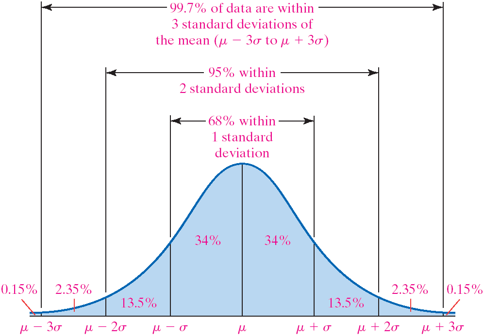
The Empirical Rule
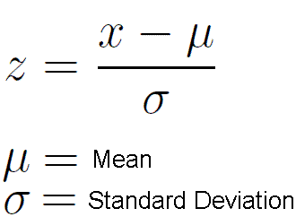
Z Scores (Standardized Score)
How many standard deviations away from the mean your value x is
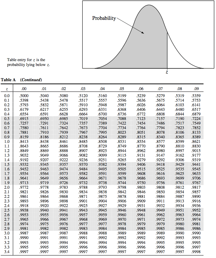
Using the Normal Table
![Probability Table entry for z is the probability lying below z. T able
A Standard normal probabilities -3.4 -3.3 -3.2 -3.1 -3.0 -2.9 -2.8 -2.7
-2.6 -2.5 -2.4 -2.3 -2.2 -2.1 -2.0 -1.9 -1.8 -1.7 —1.6 -1.5 -1.4 -1.3
-1.2 -1.1 -1.0 -0.9 -0.8 -0.7 —0.6 -0.5 -0.4 -0.3 -0.2 -0.1 -0.0 .00
0010 .0013 .0019 .0035 .0047 .0062 .0082 .0107 .0139 .0179 .0228 .0287
.0359 .0548 .0808 .1151 .1357 .1587 .1841 .2119 .2420 .2743 .3085 .3821
.4207 .4602 .01 .0003 .0005 .0013 .0018 .0025 .0045 .0104 .0136 .0174
.0222 .0281 .0351 .0436 .0537 .0655 .0793 .0951 .1131 .1335 .1562 .1814
.2090 .2389 .2709 .3050 .3409 .3783 .4168 .4562 .496() .02 .0003 .0005
.0013 .0018 .0024 .0033 .0059 .0078 .0102 .0132 .0170 .0217 .0274 .0427
.0526 .0643 .0778 .0934 .1112 .1314 .1539 .1788 .2061 .2358 .2676 .3015
.3372 .3745 .4129 .4522 .4920 .03 0003 0006 0009 0012 0017 0032 0057
0075 0099 .0129 .0166 0212 0336 0418 .0516 0630 .0764 0918 .1093 .1292
.1515 .1762 .2033 .2327 .2981 .3336 .3707 .4090 .4483 .4880 .04 .0012
.0016 .0023 .0031 .0041 .0055 .0073 .0125 .0162 .0207 .0262 .0329 .0505
.0618 .0749 .0901 .1075 .1271 .1492 .1736 .2005 .2296 .2611 .2946 .3300
.3669 .4052 .4443 .4840 .05 .0011 .0016 .0030 .0054 .0071 .0122 .0158
.0202 .0256 .0322 0401 .0495 .0606 .0735 .0885 .1056 .1251 .1469 .1711
.1977 .2266 .2578 .2912 .3264 .3632 .4013 .4801 .06 .0003 .00(M .0006
.0008 .0011 .0015 .0021 .0029 .0039 .0052 .0069 .0091 .0119 .0154 .0197
.0250 .0314 .0392 .0485 .0594 .0721 .0869 .1038 .1230 .1446 .1685 .1949
.2236 .2877 .3228 .3594 .3974 .4364 .4761 .07 .0003 .0005 .0008 .00\]1
.0015 .0021 .0028 .0038 .0051 .0068 .0089 .0116 .0150 .0192 .0244 .0307
.0384 .0475 .0582 .0708 .0853 .1020 .1210 .1423 .1660 .1922 .2514 .2843
.3192 .3557 .3936 .4325 .4721 .08 .0003 .0004 .0005 .0007 .0010 0014
0020 0027 0037 0049 .0066 .0087 .0113 .0146 .0188 0239 0301 0375 0465
0571 .0694 .0838 .1003 .1 190 .1401 .1635 .1894 .2177 .2483 .2810 .3156
.3520 .3897 .4286 .4681 .09 .0002 .0003 .0005 .0007 .0010 .0014 .0019
.0026 .0036 .0048 .0064 .0084 .0110 .0143 .0183 .0233 .0294 .0367 .0455
.0559 .0681 .0823 .0985 .1170 .1379 .1611 .1867 .2148 .2451 .2776 .3121
.3483 .3859 .4247 .4641](media/image141.png)
Practice Questions
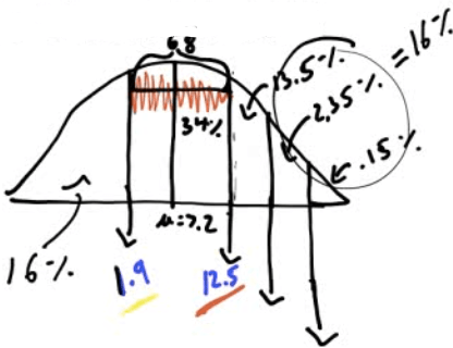
- A study of college freshmen's study habits found that the time (in hours) that college freshmen use to study each week follows a normal distribution with a mean of 7.2 hours and a standard deviation of 5.3 hours
How many hours do the students who study in the top 15% spend studying?
The middle 68%?
Top 15%: 12.5 hours
Middle 68%: 1.9 hours to 12.5 hours
- Suppose that the weight of navel oranges is normally distributed with mean of 8 ounces, and standard deviation of 1.3 ounces. And the weights of Valencia oranges is normally distributed with mean of 9 ounces, and standard deviation of 1.6 ounces
You grow a navel orange that weighs 9.5 ounces and a Valencia orange that weight 10.5 ounces, which should you enter in the giant fruit contest?
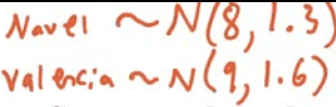
Z score for navel orange = (9.5-8)/1.3 = 1.1538
Z score for Valencia orange = (10.5-9)/1.6 = 0.9375
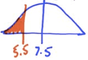
The weights of newborn children in the United States vary according to the Normal Distribution with mean 7.5 pounds and standard deviation 1.25 pounds.
What is the probability that a baby chosen at random weighs less than 5.5 pounds at birth?
- Draw a sketch
Calculate Z score
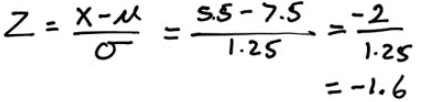
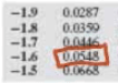
Look up probability on the normal table
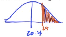
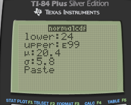
The composite score of students on the ACT college entrance examination in a recent year had a Normal distribution with mean of 20.4 and standard deviation of 5.8
What is the probability that a randomly chosen students scored 24 or higher on the ACT?
- Sketch
2ND + VARS (DISTR) ➡️ 2: normalcdf
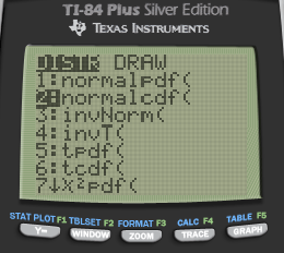
Normalcdf(lower, upper, mean, standard deviation)
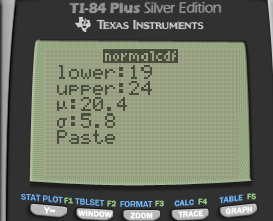
- What is the probability that a randomly chosen student scored between a 19 and a 24 on the ACT?
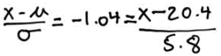
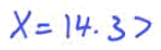
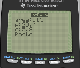
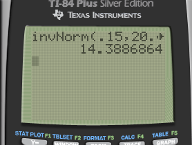
What score would someone in the 15th percentile have scored?
Sketch
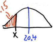
Find the z value on the normal table
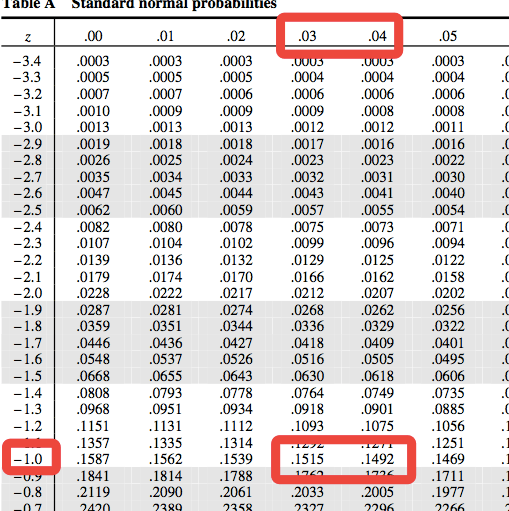
Z≈-1.035
Solve for x
Calculator: invNorm(area, mean, standard deviation)
Suppose that the mean height of men is 70 inches with a standard deviation of 3 inches. And suppose that the mean height for women is 65 inches with a standard deviation of 2.5 inches
If the heights of men and women are Normally distributed, find the probability that a randomly selected woman is taller than a randomly selected man.
- Sketch
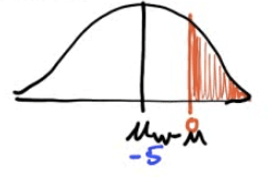
- Find the necessary information
| Mean | SD | |
|---|---|---|
| Men | 70 | 3 |
| Women | 65 | 2.5 |
| W-M | 65-70 = -5 | Sqrt(3^2+2.5^2) = 3.9 |
Calculate Z score
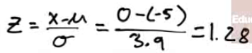
Find the probability on the table and subtract that from 1
1-0.9015 = 0.0985 = 9.85%
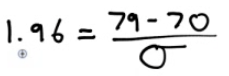
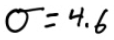
Suppose that the height (X) in inches, of adult men is a normal random variable with mean of 70 inches. If P (X>79) = 0.025
What is the standard deviation of this random normal variable?
Sketch
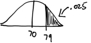
Find the z score on the calculator: invNorm(area)
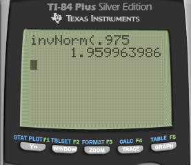
Solve for SD