Scatterplots

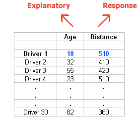
Interpreting Scatterplots
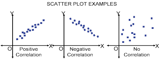
Direction: Positive or Negative
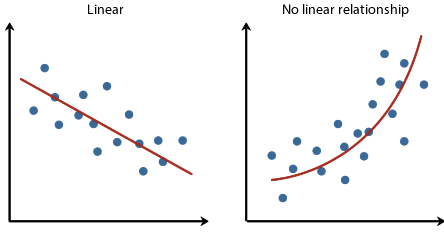
Form: Linear or Non-linear
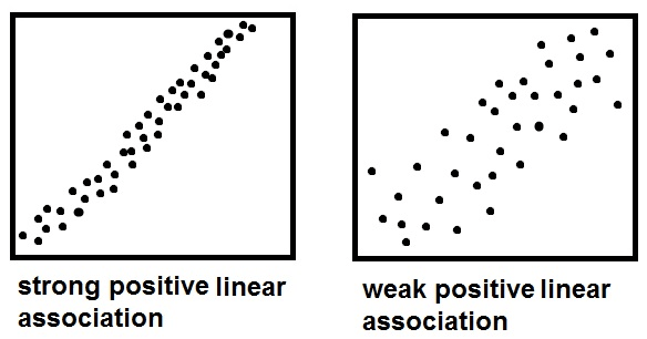
Strength: Weak, Moderate or Strong
Example
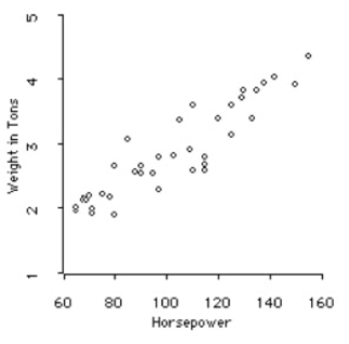
Positive, linear, strong relationship between horsepower and weight in tons.
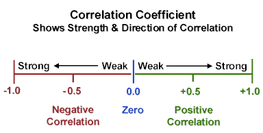
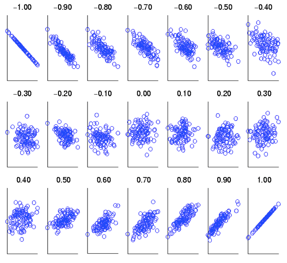
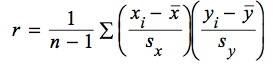
Correlation Coefficient (r)
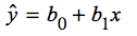
Least Squares Regression Line
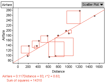
A regression line is a line that describes how y changes as x changes
Can be used to predict the value of y for a given value of x
Called the Least Squares regression line because it make the smallest sum of squares
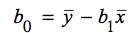
LSRL will always run through the point (mean of x, mean of y)
Formulas (hat = predicted)
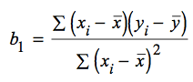

Remember to note what x and y are
Calculation
- Input data
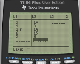
STAT➡️CALC➡️ 4:LinReg(ax+b)
LinReg(ax+b) L1, L2
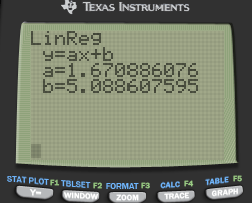
Catalog (2ND + 0) ➡️ DiagnosticOn

Do LinReg again to display r

Coefficient of Determination
R^2=r^2
Coefficient of Determination = (Correlation Coefficient)^2
Percent of the change in y that is explained by the change by the change in x / least squares regression line
From the previous example, 41.9% of the change in y can be explained by the change in x
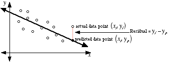
Residuals (≈error)
Residuals = observed/actual y - predicted y
Resid = y - y hat
Resid < 0: Overpredicted
Resid > 0: Underpredicted
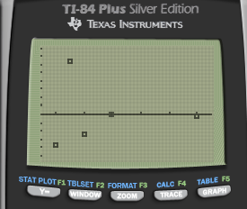
Residual Plot
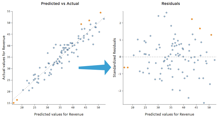
- no pattern = good fit
- Example
| X | 3 | 1 | 1.5 | 6 | 2 |
|---|---|---|---|---|---|
| Y | 10 | 3 | 14 | 15 | 6 |
| Y hat | 10.1 | 6.76 | 7.60 | 15.11 | 8.43 |
| Residuals | -0.1 | -3.76 | 6.4 | -0.11 | -2.43 |
Calculator
- Type the regression equation in L3 (y hat)
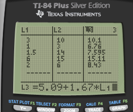
L4 = L2 - L3
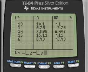
Graph L1, L4 (Residuals)
Examples
- At the summer school, one of Sarah's teachers told her that you can determine air temperature from the number of cricket chirps
What is the explanatory variable, and what it the response variable
Explanatory/independent variable: cricket chirps
Response/dependent variable: air temperature
To determine a formula, Sarah collected data on temperature and number of chirps per minute on 14 occasions. She entered the data into her calculator and did 2-Var Stats. Here are some results. Use this information to find the equation of the least-squares regression line
| Xbar | 165.8 |
|---|---|
| Sx | 32.0 |
| Ybar | 76.83 |
| Sy | 9.23 |
| r | 0.361 |
b= r * Sy / Sx = 0.104
Ybar = a + b*Xbar
a = Ybar - b*Xbar = 59.57
Yhat = 59.57 + 0.14 * x
Where y = air temperature, and x = cricket chirps
One of Sarah's data points was recorded on a particularly hot day (95F). She counted 2432 cricket chirps in one minute. What is the residual for this data point?
- Residual = Y - Yhat = 95 - (59.57 + 0.104 * 2432) = -217.498